Plot the Inferred Bayesian Boolean Network

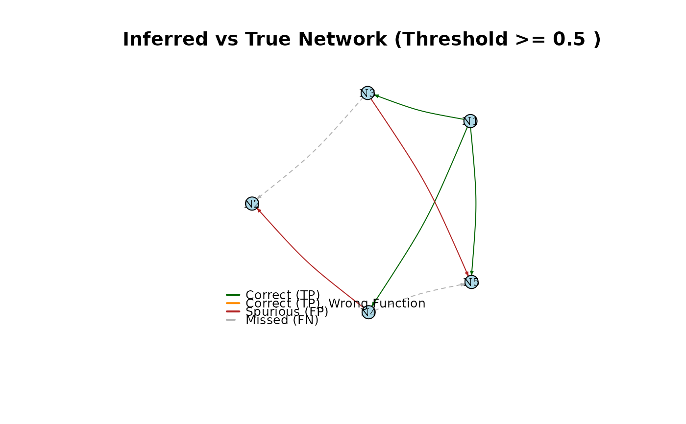
Visualizes the causal network structure inferred by the BBNI MCMC sampler. This function takes the marginal posterior probability of each directed edge and plots the network using the igraph package. Edges with posterior probabilities below the specified threshold are omitted from the plot.

Usage

plot_bbni(
  results,
  threshold = 0.5,
  node_names = NULL,
  true_network = NULL,
  ...
)

Arguments

results

The list returned by run_bbni(), containing networks and log_posterior.

threshold

Numeric. The minimum posterior probability required to draw an edge. Defaults to 0.5.

node_names

Character vector. Optional names for the nodes. Defaults to "N1", "N2", etc.

true_network

Optional square matrix representing the true network topology. If provided, edges will be color-coded to indicate true positives (along with displaying wrong function inferences), false positives, and false negatives. Purely for simulation purposes.

...

Additional graphical parameters passed to igraph::plot.igraph().

Value

An invisible igraph object.

Examples

# 1. Generate synthetic network and time-series data
set.seed(123)
true_network <- GenerateNetwork(num.node = 5)
dummy_data <- GenerateSample(true_network, SampleSize = 15)

# 2. Run BBNI sampler
prior_para <- matrix(3, nrow = 6, ncol = 2)
prior_para[6, 1] <- 2
prior_para[6, 2] <- 100

results <- run_bbni(dummy_data, prior_para = prior_para, num_update = 100)

# 3. Plot inferred network
plot_bbni(results, true_network = true_network, threshold = 0.5)