Plot MCMC Trace for BBNI — plot

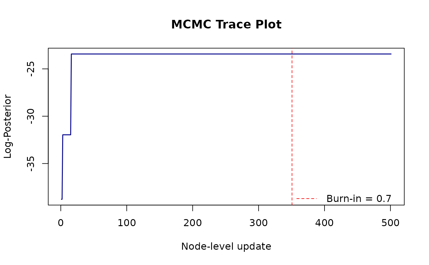
Generates a trace plot of the log-posterior values over iterations of the MCMC to visually assess convergence and stability of the executed Markov chain. Burn-in line is graphed to show when the data started to be utilized for edge-probability calculations.

Usage

plot_trace(results, every = 1)

Arguments

results: The list returned by run_bbni(), containing networks and log_posterior.
every: An integer specifying the thinning interval (sampling frequency) for plotting. Default is 1, which plots all log-posterior values. Values greater than 1 plot every every-th iteration.

Value

A base R trace plot.

Examples

# 1. Generate synthetic network and time-series data
set.seed(123)
true_network <- GenerateNetwork(num.node = 5)
dummy_data <- GenerateSample(true_network, SampleSize = 15)

# 2. Run BBNI sampler
prior_para <- matrix(3, nrow = 6, ncol = 2)
prior_para[6, 1] <- 2
prior_para[6, 2] <- 100

results <- run_bbni(dummy_data, prior_para = prior_para, num_update = 100)

# 3. Visualize MCMC results
plot_trace(results)