Getting started with Summary-statistic regional association scanning • rasSS

rasSS extends the RAS method to accept GWAS summary statistics. It replaces the per-window regressions that required individual-level data with 1-df weighted burden statistics, calculated by t_burden = w'Z / sqrt(w'Rw), using the marginal Z-scores, weights derived from a discovery set (marginal effect sizes), and an external LD reference. The resulting profile is then inputted into the original, unmodified RAS change-point detection. This vignette demonstrates a full example workflow on a small simulated chromosome.

Simulate a chromosome and an LD reference

n_snps <- 200
R_true <- matrix(0, n_snps, n_snps)
for (b in 0:3) {
  idx <- b * 50 + 1:50
  R_true[idx, idx] <- outer(1:50, 1:50, function(i, j) 0.8^abs(i - j))
}

X_ref <- sim_genotypes(2000, R_true) # external reference panel
R_emp <- cor(X_ref)
mask  <- prune_ld(R_emp, thresh = 0.2) # LD pruning mask

Discovery and target summary statistics

beta <- rep(0, n_snps)
beta[101:110] <- 0.5 # one sparse causal cluster

X_d <- sim_genotypes(1000, R_true)
X_t <- sim_genotypes(1000, R_true)
y_d <- make_pheno(X_d, beta, "continuous", seed = 2)
y_t <- make_pheno(X_t, beta, "continuous", seed = 3)

disc <- get_marginal_stats(X_d, y_d) # discovery weights w
targ <- get_marginal_stats(X_t, y_t) # target Z-scores Z

Scan with explicit window parameters

scan <- scan_ss(disc$beta, targ$z, R_emp, mask,
                skip1 = 5, skip2 = 5,
                min_window_size = 5, max_window_size = 15)

plot(scan$x, scan$y, type = "l",
     xlab = "SNP position", ylab = expression(-log[10](p)),
     main = "rasSS summary-statistic profile")
abline(v = 105, lty = 2, col = "red")  # true causal cluster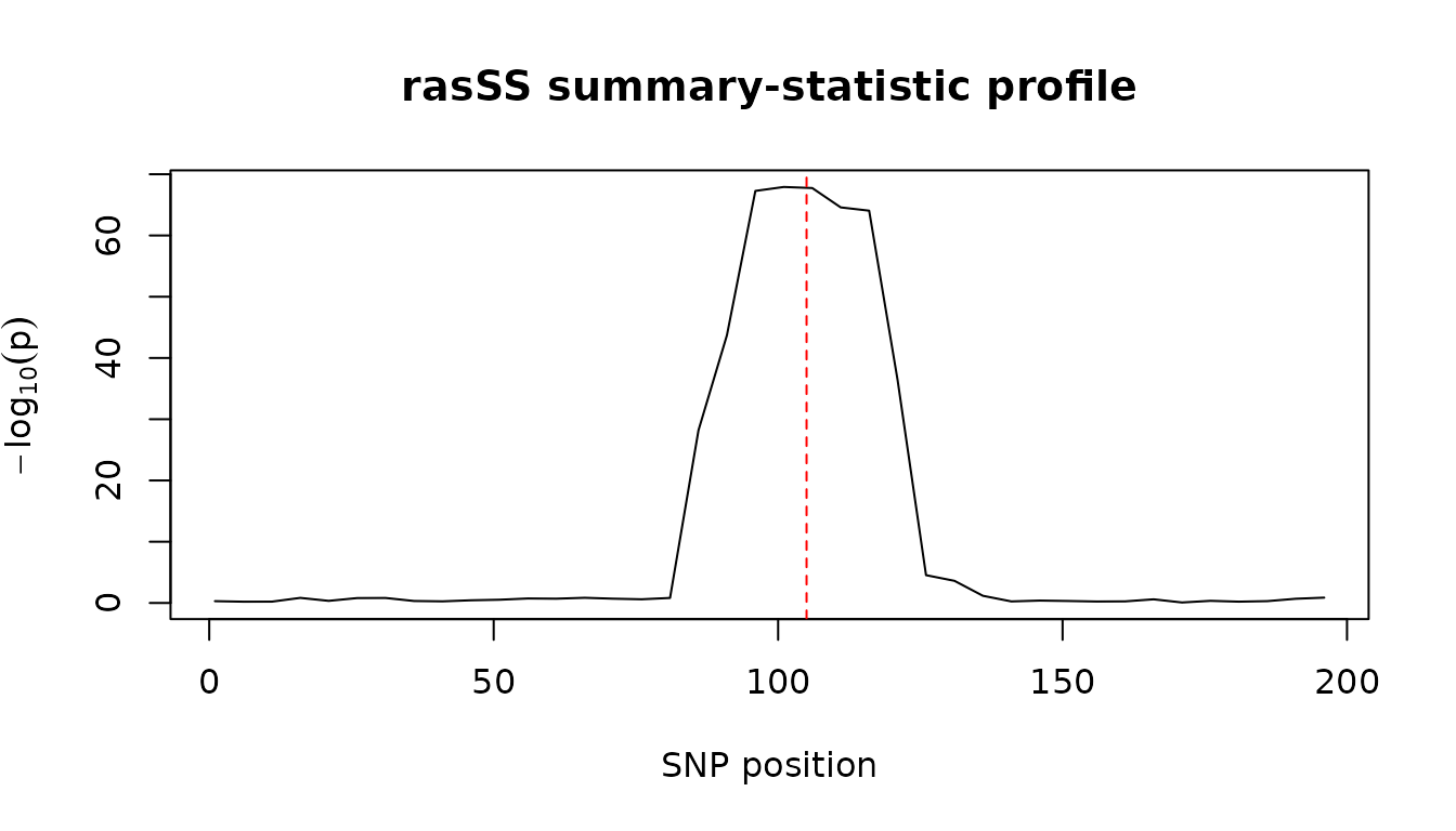

The burden statistic for a single window

win <- 96:115
t_burden(w = disc$beta[win], Z = targ$z[win], R = R_emp[win, win])
#> [1] 17.61409

Peak detection with the original RAS CPD

rasSS does not modify the original detection algorithm; the profile generated above is inputted into RAS’s own ras_detect() / ras_validate(), specifying all detection parameters.

cp <- quiet(RAS::ras_detect(x = seq_along(scan$x), y = scan$y,
                            window_size = 12, slope_check_window_size = 8,
                            slope.p.values.threshold.left = 1e-4,
                            slope.p.values.threshold.right = 1e-4))
val <- quiet(RAS::ras_validate(this.result = cp, x = seq_along(scan$x), y = scan$y,
                               this.start = 1, this.skip = 5,
                               second_window_size = 20, min_signal = 2.5,
                               p.value.threshold = 1e-3))
scan$x[val$tau_hats] # detected peak positions (SNP coordinates)
#> [1] NA

Binary traits

For case-control data, replace the marginal statistics with the Rao score version; everything else is identical as follows.

y_b   <- make_pheno(X_t, beta, "binary", seed = 4)
stat_b <- get_marginal_stats_bin(X_t, y_b)
head(stat_b$z, 3)
#> [1] -0.003737223 -0.935993213 -0.851067166

The simulation studies (small toy chromosome pilot study, paired comparison with individual-level data method, and paper-replication study) can be found on the pkgdown website under Simulations.